This talk is based on a chapter of my forthcoming book called Probably Overthinking It that is about using evidence and reason to answer questions and make better decisions. If you would like to get an occasional update about the book, please join my mailing list.
The results I reported are from 16 questions from the General Social Survey (GSS). If you would like to see the text of the questions, and answer them yourself, you can
In honor of NASA’s successful DART mission, here’s a relevant excerpt from my forthcoming book, Probably Overthinking It.
On March 11, 2022, an astronomer near Budapest, Hungary detected a new asteroid, now named 2022 EB5, on a collision course with Earth. Less than two hours later, it exploded in the atmosphere near Greenland. Fortunately, no large fragments reached the surface, and they caused no damage.
We have not always been so lucky. In 1908, a much larger asteroid entered the atmosphere over Siberia, causing an estimated 2 megaton explosion, about the same size as the largest thermonuclear device tested by the United States. The explosion flattened something like 80 million trees in an area covering 2100 square kilometers, almost the size of Rhode Island. Fortunately, the area was almost unpopulated; a similar-sized impact could destroy a large city.
These events suggest that we would be wise to understand the risks we face from large asteroids. To do that, we’ll look at evidence of damage they have done in the past: the impact craters on the Moon.
The largest crater on the near side of the moon, named Bailly, is 303 kilometers in diameter; the largest on the far side, the South Pole-Aitken basin, is roughly 2500 kilometers in diameter.
In addition to large, visible craters like these, there are innumerable smaller craters. The Lunar Crater Database catalogs nearly all of the ones larger than one kilometer, about 1.3 million in total. It is based on images taken by the Lunar Reconnaissance Orbiter, which NASA sent to the Moon in 2009.
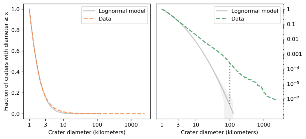
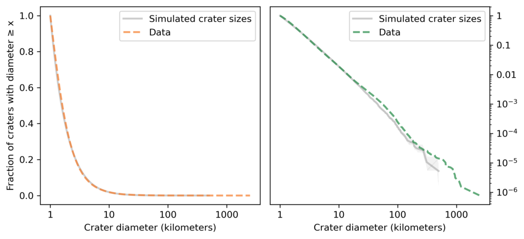
The following figures show the distribution of their sizes on a log scale, compared to a lognormal model. The left figure shows the tail distribution on a linear scale; the right figure shows the same curve on a log scale.
Since the dataset does not include craters smaller than one kilometer, I cut off the model at the same threshold. We can assume that there are many smaller craters, but with this dataset we can’t tell what the distribution of their sizes looks like.
Looking at the figure on the left, we can see a discrepancy between the data and the model between 3 and 10 kilometers. Nevertheless, the model fits the logarithms of the diameters well, so we could conclude that the distribution of crater sizes is approximately lognormal.
However, looking at the figure on the right, we can see big differences between the data and the model in the tail. In the dataset, the fraction of craters as big as 100 kilometers is about 250 per million; according to the model, it would be less than 1 per million. The dotted line in the figure shows this difference.
Going farther into the tail, the fraction of craters as big as 1000 kilometers is about 3 per million; according to the model, it would be less than one per trillion. And the probability of a crater as big as the South Pole-Aitken basin is about 50 per sextillion.
If we are only interested in craters less than 10 kilometers in diameter, the lognormal model might be good enough. But for questions related to the biggest craters, it is way off.
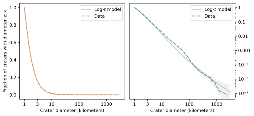
The following figure shows the distribution of crater sizes again, compared to a log-t model [which is the abbreviated name I use for a Student-t distribution on a log scale].
The figure on the left shows that the model fits the data well in the middle of the distribution, a little better than the lognormal model. The figure on the right shows that the log-t model fits the tail of the distribution substantially better than the lognormal model.
It’s not perfect: there are more craters near 100 km than the model expects, and fewer craters larger than 1000 km. As usual, the world is under no obligation to follow simple rules, but this model does pretty well.
We might wonder why. To explain the distribution of crater sizes, it helps to think about where they come from. Most of the craters on the Moon were formed during a period in the life of the solar system called the “Late Heavy Bombardment”, about 4 billion years ago. During this period, an unusual number of asteroids were displaced from the asteroid belt – possibly by interactions with large outer planets – and some of them collided with the Moon.
We assume that some of them also collided with the Earth, but none of the craters they made still exist; due to plate tectonics and volcanic activity, the surface of Earth has been recycled several times since the Late Heavy Bombardment.
But the Moon is volcanically inert and it has no air or water to erode craters away, so its craters are visible now in almost the same condition they were 4 billion years ago (with the exception of some that have been disturbed by later impacts and lunar spacecraft).
Asteroids
As you might expect, there is a relationship between the size of an asteroid and the size of the crater it makes: in general, a bigger asteroid makes a bigger crater. So, to understand why the distribution of crater sizes is long-tailed, let’s consider the distribution of asteroid sizes.
The Jet Propulsion Laboratory (JPL) and NASA provide data related to asteroids, comets and other small bodies in our solar system. From their Small-Body Database, I selected asteroids in the “main asteroid belt” between the orbits of Mars and Jupiter.
There are more than one million asteroids in this dataset, about 136,000 with known diameter. The largest are Ceres (940 kilometers in diameter), Vesta (525 km), Pallas (513 km), and Hygeia (407 km). The smallest are less than one kilometer.
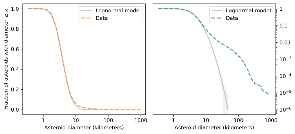
The following figure shows the distribution of asteroid sizes compared to a lognormal model.
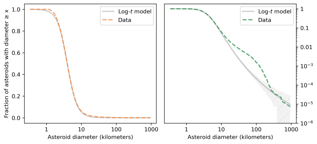
As you might expect by now, the lognormal model fits the distribution of asteroid sizes in the middle of the range, but it does not fit the tail at all. Rather than belabor the point, let’s get to the log-t model, as shown in the following figure.
On the left, we see that the log-t model fits the data well near the middle of the range, except possibly near 1 kilometer.
On the right, we see that the model does not fit the tail of the distribution particularly well: there are more asteroids near 100 km than the model predicts. So the distribution of asteroid sizes does not strictly follow a log-t distribution. Nevertheless, it is clearly longer-tailed than a lognormal distribution, and we can use it to explain the distribution of crater sizes, as I’ll show in the next section.
Origins of Long-Tailed Distributions
One of the reasons long-tailed distributions are common in natural systems is that they are persistent; for example, if a quantity comes from a long-tailed distribution and you multiply it by a constant or raise it to a power, the result follows a long-tailed distribution.
Long-tailed distributions also persist when they interact with other distributions. When you add together two quantities, if either comes from a long-tailed distribution, the sum follows a long-tailed distribution, regardless of what the other distribution looks like. Similarly, when you multiply two quantities, if either comes from a long-tailed distribution, the product usually follows a long-tailed distribution. This property might explain why the distribution of crater sizes is long-tailed.
Empirically – that is, based on data rather than a physical model – the diameter of an impact crater depends on the diameter of the projectile that created it, raised to the power 0.78, and on the impact velocity raised to the power 0.44. It also depends on the density of the asteroid and the angle of impact.
As a simple model of this relationship, I’ll simulate the crater formation process by drawing asteroid diameters from the distribution in the previous section and drawing the other factors – density, velocity, and angle – from a lognormal distribution with parameters chosen to match the data. The following figure shows the results from this simulation along with the actual distribution of crater sizes.
In the center of the distribution (left) and in the tail (right), the simulation results are a good match for the data. This example suggests that the distribution of crater sizes can be explained by the relationship between the distributions of asteroid sizes and other factors like velocity and density.
In turn, there are physical models that might explain the distribution of asteroid sizes. Our best current understanding is that the asteroids in the asteroid belt were formed by dust particles that collided and stuck together. This process is called “accretion”, and simple models of accretion processes can yield long-tailed distributions.
So it may be that craters are long-tailed because of asteroids, and asteroids are long-tailed because of accretion.
In The Fractal Geometry of Nature, Benoit Mandelbrot proposes what he calls a “heretical” explanation for the prevalence of long-tailed distributions in natural systems: there may be only a few systems that generate long-tailed distributions, but interactions between systems might cause them to propagate.
He suggests that data we observe are often “the joint effect of a fixed underlying true distribution and a highly variable filter”, and “a wide variety of filters leave their asymptotic behavior unchanged”.
The long tail in the distribution of asteroid sizes is an example of “asymptotic behavior”. And the relationship between the size of an asteroid and the size of the crater it makes is an example of a “filter”. In this relationship, the size of the asteroid gets raised to a power and multiplied by a “highly-variable” lognormal distribution. These operations change the location and spread of the distribution, but they don’t change the shape of the tail.
When Mandelbrot wrote in the 1970s, this explanation might have been heretical, but now long-tailed distributions are more widely known and better understood. What was heresy then is orthodoxy now.
On September 25, 2022, Eliud Kipchoge ran the Berlin Marathon in 2:01:09, breaking his own world record by 30 seconds and taking another step in the progression toward a two-hour marathon.
In a previous article, I noted that the marathon record speed since 1970 has been progressing linearly over time, and I proposed a model that explains why we might expect it to continue. Based on a linear extrapolation of the data so far, I predicted that someone would break the two hour barrier in 2036, plus or minus five years.
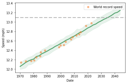
Now it is time to update my predictions in light of the new record. The following figure shows the progression of world record speed since 1970 (orange dots), a linear fit to the data (green line) and a 90% predictive confidence interval (shaded area).
This model predicts that we will see a two-hour marathon in 2035 plus or minus 6 years. Since the last two points are above the long-term trend, we might expect to cross the finish line on the early end of that range.
If you like this sort of thing, you will like my forthcoming book, called Probably Overthinking It, which is about using evidence and reason to answer questions and guide decision making. If you would like to get an occasional update about the book, please join my mailing list.
I’m working on a book called Probably Overthinking It that is about using evidence and reason to answer questions and guide decision making. If you would like to get an occasional update about the book, please join my mailing list.
In the previous article, I used data from the General Social Survey (GSS) to show that polarization on an individual level has increased since the 1970s, but not by very much. I identified fifteen survey questions that distinguish conservatives and liberals; for each respondent, I estimated the number of conservative responses they would give to these questions.
Since the 1970s, the average number of conservative responses had decreased consistently. The spread of the distribution has increased slightly, but if we quantify the spread as a mean absolute difference, here’s what it means: in 1986, if you chose two people at random and asked them the fifteen questions, they would differ on 3.4 questions, on average. If you repeated the experiment in 2016, they would differ by 3.6.
That is not a substantial change.
But even without polarization at the individual level, there can be polarization at the level of political parties. So that’s what this article is about.
Here’s an overview of the results:
In the 1970s, there was not much difference between Democrats and Republicans. On average, their answers to the fifteen questions were about the same.
Since then, both parties have moved to the left (and nonpartisans, too). But the Democrats have moved faster, so the gap between the parties has increased.
Although it is tempting to interpret these results as a case of Democrats careening off to the left, that is a misleading way to tell the story, because it sounds like we are following a group of people over time. The groups we call Democrats and Republicans are not the same groups of people over time. The composition of the groups changes due to:
Generational replacement: In the conveyor belt of demography, when old people die, they are replaced by young people, and
Partisan sorting: No one is born Democrat or Republican; rather, they choose a party (or not) at some point in their lives, and this sorting process has changed over time.
These two factors explain the increasing ideological difference between Democrats and Republicans: polarization between the parties is not caused by people changing their minds; it is caused by changes in the composition of the groups.
Let me show you what I mean.
The race to the bottom
Each GSS respondent was asked “Generally speaking, do you usually think of yourself as a Republican, Democrat, Independent, or what?” Their responses were coded on a 7-point scale, but for simplicity, I’ve reduced it to three: Republican, Democrat, and Nonpartisan (which I think is more precise than “Independent”).
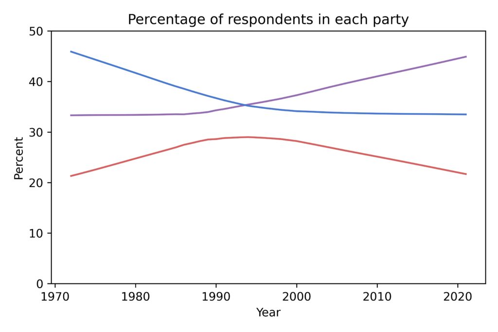
The following figure shows how the percentage of respondents in each group has changed over time:
The percentage of Democrats was decreasing until 2000; the percentage of Republicans has decreased since. But there is no sign of increasing partisanship. In fact, the percentage of Nonpartisans has increased to the point where they are now the plurality.
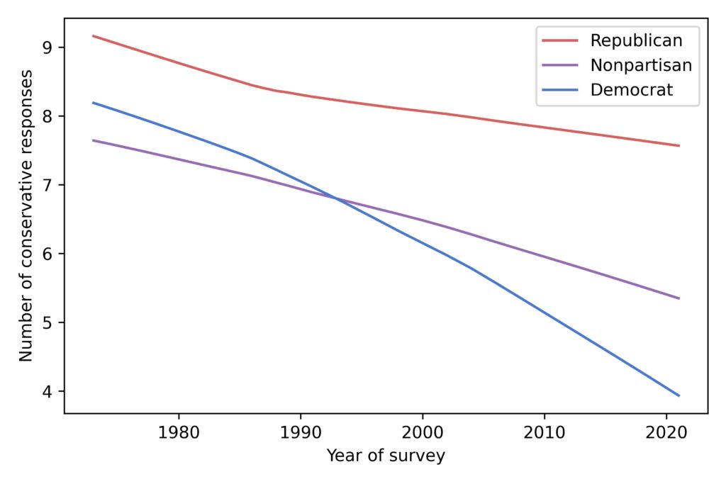
Now let’s see what these groups believe, on average. The following figure shows the estimated number of conservative responses for each group over time.
In the 1970s, there was not much difference between Democrats and Republicans. In fact, Democrats were more conservative than Nonpartisans. Since then, all three groups have moved to the left; that is, they give more liberal responses to the fifteen questions. But Democrats have moved faster than the other groups.
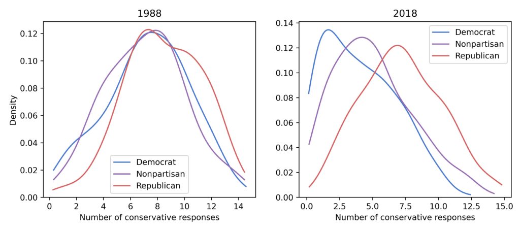
These are just averages; we can get a better view of what’s happening by looking at the distributions. The following figure shows the distribution of responses for the three groups in 1988 and 2018.
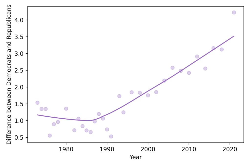
In 1988, the three groups were almost indistinguishable. In 2018, they still overlap substantially, but Democrats have shifted farther to the left than the other two groups. As a result, the difference in the means between the groups has increased, as shown in this figure:
Now it might be clearer why I chose 1988, which is close to the lowest point in the long-term trend, and 2018, which is the most recent point that is not subject to the effects of data collection during the pandemic.
It might be tempting, especially for conservative Republicans, to interpret these graphs as a case of Democrats going off the rails, but I think that’s misleading. Again, these groups are not made up of the same people over time, so this is not a story about people whose views are changing. It is a story about groups whose composition is changing.
Partisan sorting
In the 1970s, there was not much difference between Democrats and Republicans, in term of their political views. Now, in the 2020s, there is. So what changed?
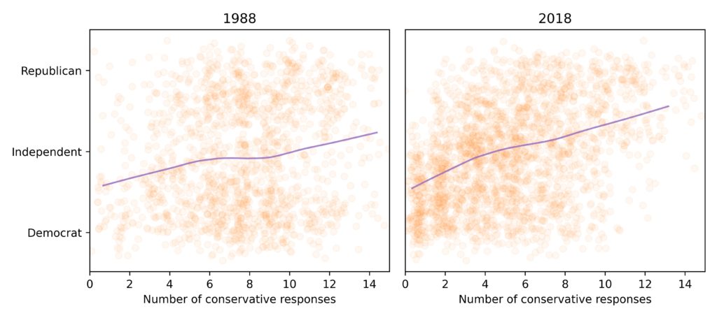
To find out, let’s look at the relationship between conservatism, as measured by responses to the fifteen questions, and party affiliation. The following figure shows a scatter plot of these values in 1988 and 2018. The purple lines show a smoothed average of party affiliation as a function of conservatism.
In 1988, the relationship between these values was weak. Someone who gave conservative responses to the questions was only marginally more likely to identify as Republican; someone who gave liberal responses was only marginally more likely to identify as Democrat.
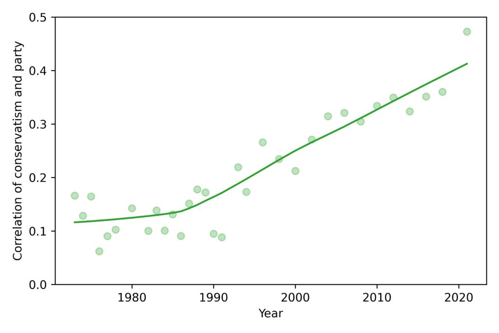
Since then, the relationship has grown stronger. The following figure shows the correlation between these values over time:
In 2018, the correlation was about 0.15, which is quite weak; in 2018 it was almost 0.4. That’s substantially higher, but it is still not a strong correlation. As you can see in the scatter plots, there are still people with liberal views who call themselves Republicans (even if Republicans have different names for them) and people with conservative views who consider themselves Democrats.
This is why I think it’s misleading to say that Democrats have moved to the left; rather, people have sorted themselves into parties according to their beliefs, at least more than they used to.
Consider this analogy: In my first year of middle school, we all took the same physical education class, so we all played the same sports. During some weeks, everyone played basketball; during other weeks, everyone wrestled. So that year, the wrestlers and the basketball players were the same height, on average.
The next year, we got to choose which sports to play. As you would expect, taller people were more likely to choose basketball and shorter people were more likely to wrestle. So, all of a sudden, the basketball players were taller than the wrestlers, on average.
Does that mean the basketball players got taller and the wrestlers got shorter? That would not be a reasonable interpretation, because they were not the same groups of people. The increased difference between the groups was entirely because of how they sorted themselves out.
Let’s see if the same is true for Democrats and Republicans.
Getting counterfactual
How much of the increased difference since the 1980s can be explained by partisan sorting? To answer that question, I used ordinal logistic regression to model the relationship between conservative views and party affiliation for each year of the survey. Then I used the model to simulate the sorting process under two scenarios:
With observed changes partisan sorting: In this version, I used the model from each year to simulating the sorting process each year — so we expect the results to be similar to the actual data.
With no change in partisan sorting: In this version, I built a model using data from the low correlation period (1973 to 1985) — then I used this model to simulate the sorting process for every year.
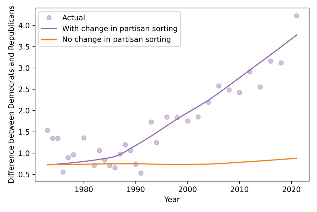
The second scenario is meant to simulate what would have happened if the sorting process had not changed. The following figure shows the results.
When the model includes the observed changes in partisan sorting, it matches the data well, which shows that the model includes the essential features that replicate the observed increase in the difference between Democrats and Republicans.
When we run the model with no increase in partisan sorting, there is no increase in the difference between Democrats and Republicans. This result shows that the observed increase in partisan sorting is sufficient to explain the entire increase in difference between the parties.
Alignment is not polarization
Compared to the 1980s, there is more alignment now between political ideology and political parties. Liberals are more likely to identify as Democrats and conservatives are more likely to identify as Republicans. As a result, the parties are more differentiated now than they were.
This alignment might not be a bad thing. In a two party system, it might be desirable if one party represents a more conservative world view than the other. If voters have only two options, the options should be different in ways voters care about. That way, at least, you know what you are voting for. The alternative, with no substantial difference between parties, is a recipe for voter frustration and disengagement.
Of course, there are problems with extreme partisanship. But I don’t think a moderate level of alignment — which is what we have — is necessarily a problem.
I’m working on a book called Probably Overthinking It that is about using evidence and reason to answer questions and guide decision making. If you would like to get an occasional update about the book, please join my mailing list.
I’m a little tired of hearing about how polarized we are, partly because I suspect it’s not true and mostly because it is “not even wrong” — that is, not formulated as a meaningful hypothesis.
To make it meaningful, we can start by distinguishing “mass polarization“, which is movement of popular attitudes toward the extremes, from polarization at the level of political parties. I’ll address mass polarization in this article and the other kind in the next.
The distribution of attitudes
To see whether popular opinion is moving toward the extremes, I’ll use data from the General Social Survey (GSS). And I’ll build on the methodology I presented in this previous article, where I identified fifteen questions that most strongly distinguish conservatives and liberals.
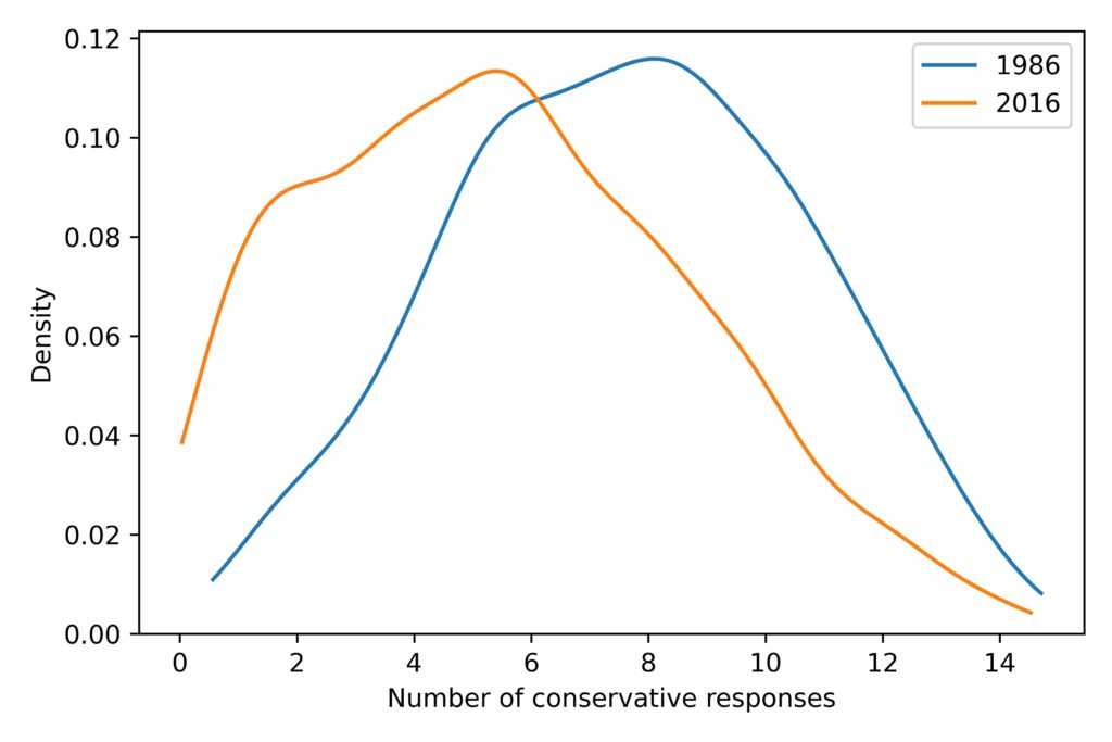
Not all respondents were asked all fifteen questions, but with some help from item response theory, I estimated the number of conservative responses each respondent would give, if they had been asked. From that, we can estimate the distribution of responses during each year of the survey. For example, here’s a comparison of distributions from 1986 and 2016:
First, notice that the distributions have one big mode near the middle, not two modes at the extremes. That means that most people choose a mixture of liberal and conservative responses to the questions; the people at the extremes are a small minority.
Second, the distribution shifted to the left during this period. In 1986, the average number of conservative responses was 7.6; in 2016, it was 5.5.
Now, let’s see what happened during the other years.
It’s just a jump to the left
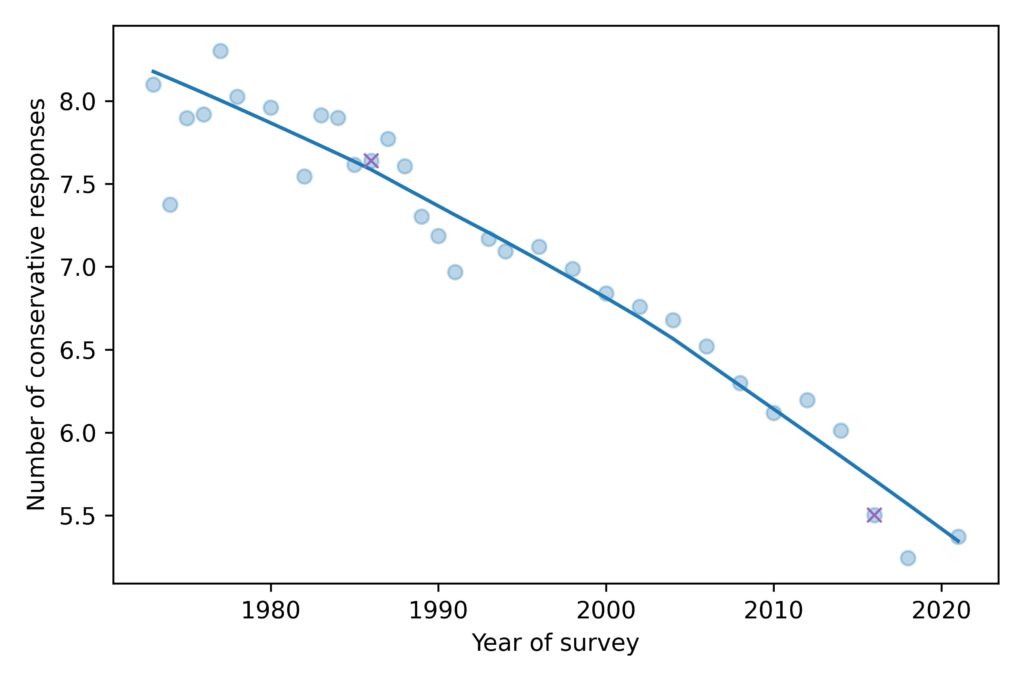
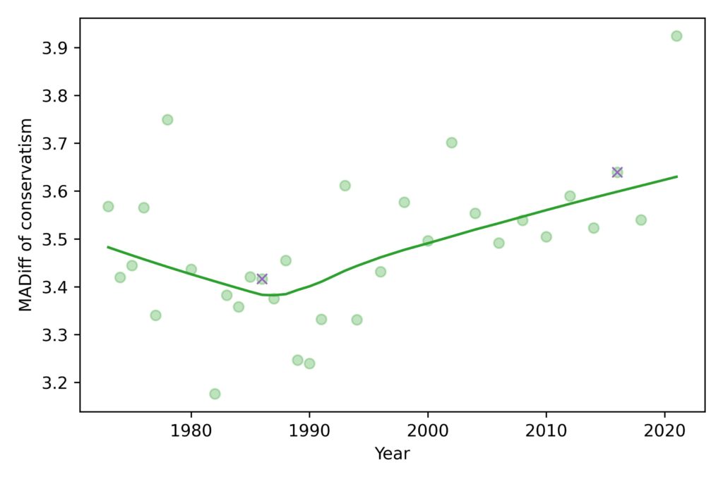
To summarize how the distribution of responses has changed over time, we’ll look at the mean, standard deviation, and mean absolute difference. Here’s the mean for each year of the survey:
The average level of conservatism, as measured by the fifteen questions, has been declining consistently for the duration of the GSS, almost 50 years.
The ‘x’ markers highlight 1986 and 2016, the years I chose in the previous figure. So we can see that these years are not anomalies; they are both close to the long-term trend.
Measuring polarization
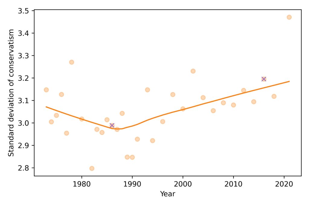
Now, to see if we are getting more polarized, let’s look at the standard deviation of the distribution over time:
The spread of the distribution was decreasing until the 1980s and has been increasing ever since. The value for 2021 is substantially above the long term trend, but it’s too early to say whether that’s a real change in polarization or an artifact of pandemic-related changes in data collection.
Again, the ‘x’ markers highlight the years I chose, and show why I chose them: they are close to the lowest and highest points in the long-term trend.
So there is some evidence of popular polarization. In fact, using standard deviation to quantify polarization might underestimate the size of the change, because the tail of the most recent distribution is compressed at the left end of the scale.
However, it is hard to interpret a change in standard deviation in practical terms. It was 3.0 in 1986 and 3.2 in 2016; is that a big change? I don’t know.
Don’t get MAD, get mean average difference
We can mitigate the effect of compression and help with interpretation by switching to a different measure of spread, mean absolute difference, which is the average size of the differences between pairs of people. Here’s how this measure has changed over time:
The mean absolute difference (MADiff) follows the same trend as standard deviation. It decreased until the 1980s and has increased ever since. It was 3.4 in 1986, which means that if you chose two people at random and asked them the fifteen questions, they would differ on 3.4 questions, on average. If you repeated the experiment in 2016, they would differ by 3.6.
This measure of polarization suggests that the increase since the 1980s has not been big enough to make much of a difference. If civilized society can survive when people disagree on 3.4 questions, it’s hard to imagine that the walls will come tumbling down when they disagree on 3.6.
In conclusion, it doesn’t look like mass polarization has changed much in the last 50 years, and certainly not enough to justify the amount of coverage it gets.
But there is another kind of polarization, at the level of political parties, that might be a bigger problem. I’ll get to that in the next article.
In 2019 I presented a talk at SciPy where I showed that support for gun control has been declining in the U.S. since about 1999. And, contrary to what many people believe, it is lowest among millennials and Gen Z.
Those results were based on data from the General Social Survey up to 2018. Now that the data from 2021 is available, I’ve run the same analysis and I can report:
Support for gun control has continued to decline, and
Among young adults it has reached a new low.
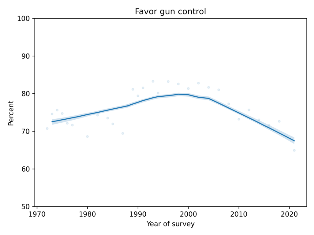
The following figure shows the fraction of GSS respondents who said that they would favor “a law which would require a person to obtain a police permit before he or she could buy a gun.”
Support for this form of gun control increased between 1972 and 1999, and has been decreasing ever since.
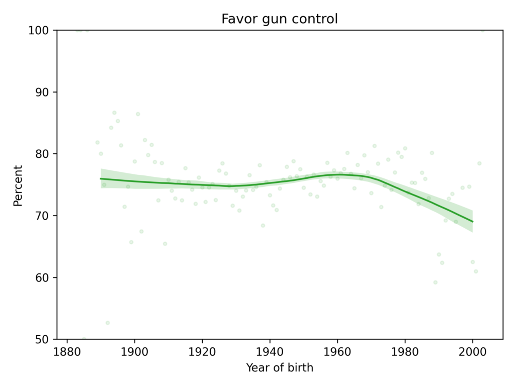
The following figure shows the results from the same question plotted over year of birth.
People born between 1890 and 1970 supported gun control at about the same level. More recent generations — including millennials and Gen Z — are substantially less likely to support gun control.
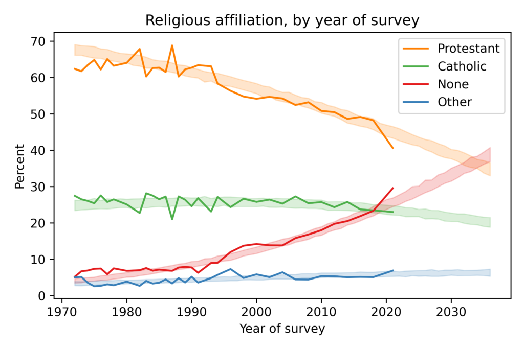
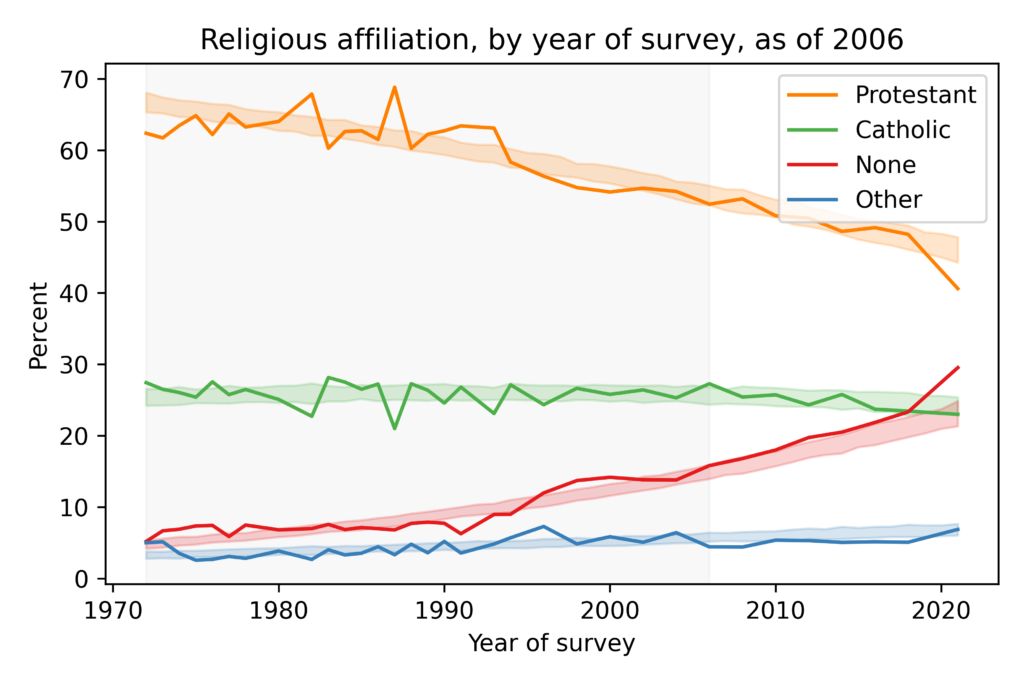
In this figure, the solid lines show estimated proportions of each religious affiliation from 1972 to 2021. Since the early 1990s, the proportion of Protestants has been declining and the proportion of people with no religious affiliation has been increasing. Catholicism has declined slightly and other religions have increased slightly.
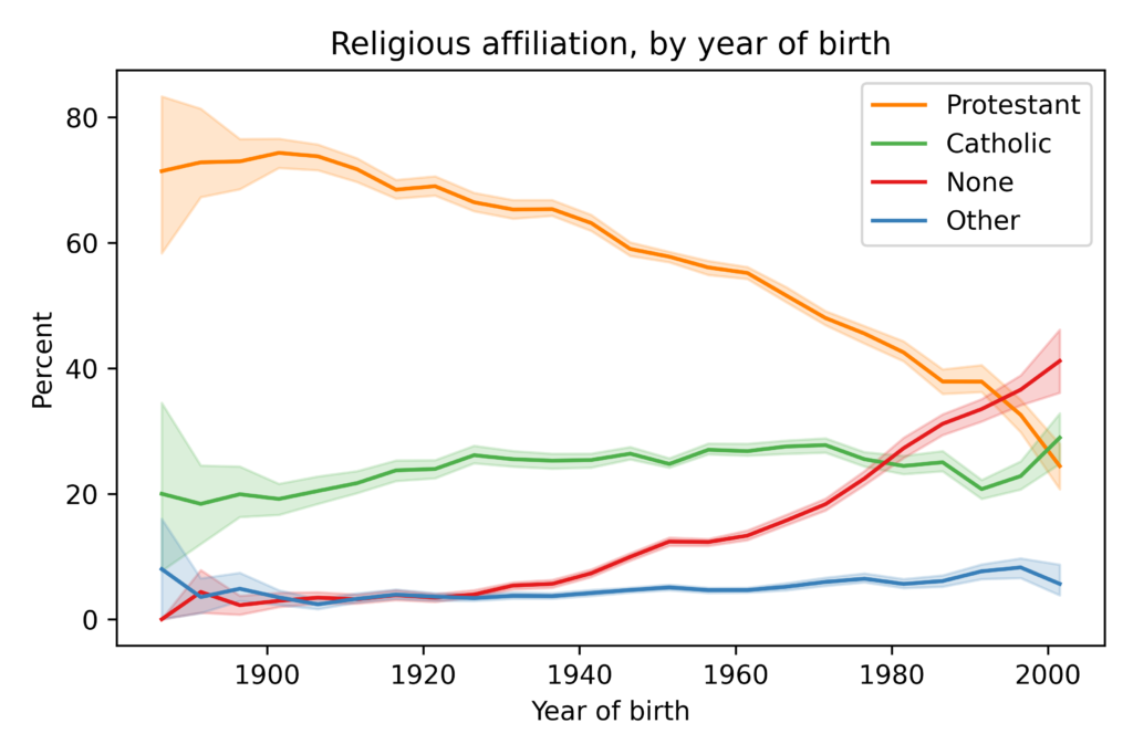
The shaded areas show results from a model I used to fit past data and forecast future changes. The model predicts that “Nones” will overtake Protestants in the 2030s. The primary cause of these changes is generational replacement: as older people die, they are replaced by young people who are less likely to be religious. The following figure shows the proportion of each religious tradition as a function of year of birth:
Among people born around 1900, nearly all were Protestant or Catholic; few belonged to another religion or none. Among people born around 2000, the plurality have no religious affiliation; Protestants and Catholics are statistically tied for second.
In general, forecasting social phenomena is hard because things change. However, generational replacement is relatively predictable. To see how predictable, let’s see what would have happened if we used the same method to generate predictions 15 years ago:
Predictions made in 2006 (using only the data in the shaded area) would have been pretty good. We would have underestimated the growth of the Nones, but the predictions for the other groups would have been accurate. So we have reason to think 15-year predictions based on current data are reliable.
If you want details, the model is multinomial logistic regression using two features: year of birth and year of survey. It is based on the assumption that (1) the distribution of ages will not change substantially over the next 15 years, and (2) most people don’t change religious affiliation as adults, or if they do, the resulting net flow between affiliations is small.
I have news. I finished the last two chapters of Probably Overthinking It last week and sent a complete draft of the book off for technical review. Yay!
In the last chapter, I used some methodology I thought was worth reporting, but too technical for the book, which is intended for an intelligent general audience. So I’ve started a public site for the book, where I will post technical details from each chapter and maybe some of the material that I decided to cut.
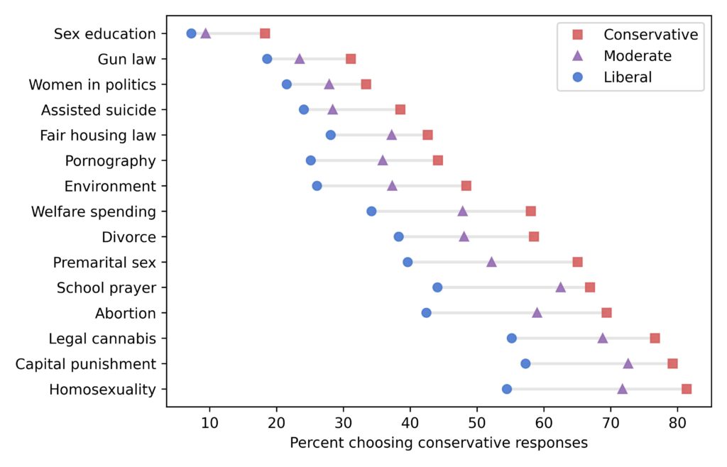
The last chapter is about changes in political beliefs over the last 50 years, particularly along the axis of liberal and conservative views. I found 15 questions in the General Social Survey (GSS) where liberals and conservatives give different answers by the widest margin. The following figure shows the topics, which will come as no surprise, and the differences between the groups.
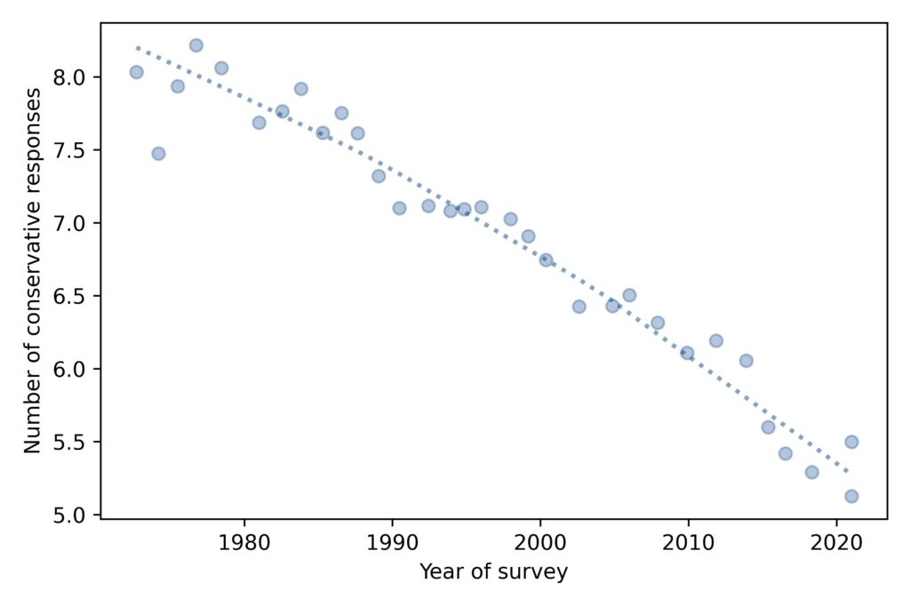
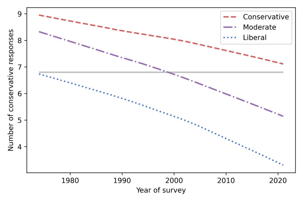
Based on the answers to these questions, I estimate a score for each respondent that quantifies how conservative their beliefs are. By this measure, people have been getting more liberal, pretty consistently, for the last 50 years:
And it’s not just liberals becoming more liberal. People who consider themselves conservative are more liberal than they used to be, too.
That gray line is at 6.8 conservative responses, which was the expected level in 1974 among people who called themselves liberal.
Now, suppose you take a time machine back to 1974, find an average liberal, and bring them to the turn of the millennium. Based on their survey responses, they would be indistinguishable from the average moderate in 2000.
And if you bring them to 2021, their quaint 1970s liberalism would be almost as far to the right as the average conservative.
I thought I would be done this week, but it looks like there will be one more chapter. If you don’t know, I am working on a book that includes updated articles from this blog, plus new examples, and pulls the whole thing together. So far, it’s going well. I have consistently finished one chapter per month and I am almost done.
The problem is that several times a chapter has mitosed (it’s a word) into multiple chapters. In the most extreme case, the material I thought would be one chapter turned into four, and I think I’m going to cut one of them.
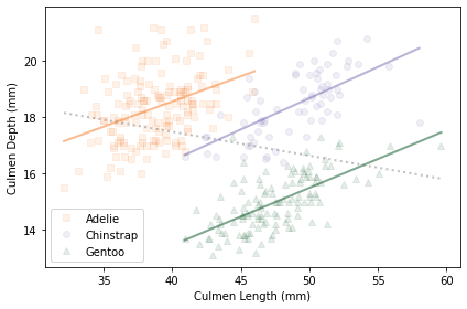
Most recently, what I thought was the last chapter has turned into two. The first is about Simpson’s paradox, including this mandatory example from the ubiquitous penguin dataset:
The new chapter is about Overton’s window. Fortunately, before the mitosis, I had written a substantial chunk of it, so I think I can finish it in less than a month.
Until then, if you would like to get infrequent email announcements about the book, please sign up below. I’ll let you know about milestones, promotions, and other news, but not more than one email per month. I will not share your email or use this list for any other purpose.
This article is an excerpt from my book Probably Overthinking It, to be published by the University of Chicago Press in early 2023. This book is intended for a general audience, so I explain some things that might be familiar to readers of this blog – and I leave out the Python code. After the book is published, I will post the Jupyter notebooks with all of the details! If you would like to receive infrequent notifications about the book (and possibly a discount), please sign up for this mailing list.
Suppose you are the ruler of a small country where the population is growing quickly. Your advisers warn you that unless growth slows down, the population will exceed the capacity of the farms and the peasants will starve.
The Royal Demographer informs you that the average family size is currently 3; that is, each woman in the kingdom bears three children, on average. He explains that the replacement level is close to 2, so if family sizes decrease by one, the population will stabilize at a sustainable size.
One of your advisors asks: “What if we make a new law that says every woman has to have fewer children than her mother?”
It sounds promising. As a benevolent despot, you are reluctant to restrict your subjects’ reproductive freedom, but it seems like such a policy could be effective at reducing family size with minimal imposition.
“Make it so,” you say.
Twenty-five years later, you summon the Royal Demographer to find out how things are going.
“Your Highness,” they say, “I have good news and bad news. The good news is that adherence to the new law has been perfect. Since it was put into effect, every woman in the kingdom has had fewer children than her mother.”
“That’s amazing,” you say. “What’s the bad news?”
“The bad news is that the average family size has increased from 3.0 to 3.3, so the population is growing faster than before, and we are running out of food.”
“How is that possible?” you ask. “If every woman has fewer children than her mother, family sizes have to get smaller, and population growth has to slow down.”
Actually, that’s not true.
In 1976, Samuel Preston, a demographer at the University of Washington, published a description of this apparent paradox: “A major intergenerational change at the individual level is required in order to maintain intergenerational stability at the aggregate level.”
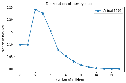
To make sense of this, I’ll use the distribution of fertility in the United States (rather than your imaginary island). Every other year, the Census Bureau surveys a representative sample women in the United States and asks, among other things, how many children they have ever born. To measure completed family sizes, they select women aged 40-44 (of course, some women have children in their forties, so these estimates might be a little low).
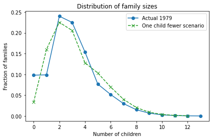
I used the data from 1979 to estimate the distribution of family sizes at the time of Preston’s paper. Here’s what it looks like.
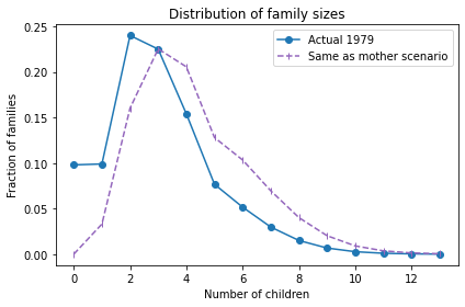
The average total fertility was close to 3. Starting from this distribution, what would happen if every woman had the same number of children as her mother? A woman with 1 child would have only one grandchild; a woman with 2 children would have 4 grandchildren; a woman with 3 children would have 9 grandchildren, and so on. In the next generation, there would be more big families and fewer small families.
Here’s what the distribution would look like in this “Same as mother” scenario.
The net effect is to shift the distribution to the right. If this continues, family sizes would increase quickly and population growth would explode.
So what happens in the “One child fewer” scenario? Here’s what the distribution looks like:
Bigger families are still overrepresented, but not as much as in the “Same as mother” scenario. The net effect is an increase is average fertility from 3 to 3.3.
As Preston explained, “under current [1976] patterns a woman would have to bear an average of almost two children fewer than … her mother merely to keep population fertility rates constant from generation to generation”. One child fewer was not enough!
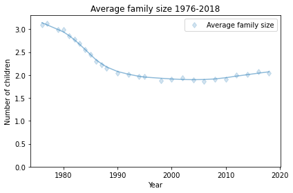
As it turned out, the next generation in the U.S. had 2.3 fewer children than their mothers, on average, which caused a steep decline in average fertility:
Average fertility in the U.S. has been close to 2 since about 1990, although it might have increased in the last few years (keeping in mind that the women interviewed in 2018 had most of their children 10-20 years earlier).
Preston concludes, “Those who exhibit the most traditional behavior with respect to marriage and women’s roles will always be overrepresented as parents of the next generation, and a perpetual disaffiliation from their model by offspring is required in order to avert an increase in traditionalism for the population as a whole.”
So, if you have fewer children than your parents, don’t let anyone say you are selfish; you are doing your part to avert population explosion!
My thanks to Prof. Preston for comments on a previous version of this article.
If you would like to get infrequent email announcements about my book, please sign up below. I’ll let you know about milestones, promotions, and other news, but not more than one email per month. I will not share your email or use this list for any other purpose.