I am excited to announce that I have started work on a third edition of Think Stats, to be published by O’Reilly Media in 2025. At this point the content is mostly settled, and I am revising chapters to get them ready for technical review.

If you want to start reading now, the current draft is here.

What’s new?

For the third edition, I started by moving the book into Jupyter notebooks. This change has one immediate benefit – you can read the text, run the code, and work on the exercises all in one place. And the notebooks are designed to work on Google Colab, so you can get started without installing anything.

The move to notebooks has another benefit – the code is more visible. In the first two editions, some of the code was in the book and some was in supporting files available online. In retrospect, it’s clear that splitting the material in this way was not ideal, and it made the code more complicated than it needed to be. In the third edition, I was able to simplify the code and make it more readable.

Since the last edition was published, I’ve developed a library called empiricaldist that provides objects that represent statistical distributions. This library is more mature now, so the updated code makes better use of it.

When I started this project, NumPy and SciPy were not as widely used, and Pandas even less, so the original code used Python data structures like lists and dictionaries. This edition uses arrays and Pandas structures extensively, and makes more use of functions these libraries provide. I assume readers have some familiarity with these tools, but I explain each feature when it first appears.

The third edition covers the same topics as the original, in almost the same order, but the text is substantially revised. Some of the examples are new; others are updated with new data. I’ve developed new exercises, revised some of the old ones, and removed a few. I think the updated exercises are better connected to the examples, and more interesting.

Since the first edition, this book has been based on the thesis that many ideas that are hard to explain with math are easier to explain with code. In this edition, I have doubled down on this idea, to the point where there is almost no mathematical notation, only code.

Overall, I think these changes make Think Stats a better book. To give you a taste, here’s an excerpt from Chapter 12: Time Series Analysis.

Multiplicative Model

The additive model we used in the previous section is based on the assumption that the time series is well modeled as the sum of a long-term trend, a seasonal component, and a residual component – which implies that the magnitude of the seasonal component and the residuals does not vary over time.

As an example that violates this assumption, let’s look at small-scale solar electricity production since 2014.

solar = elec["United States : small-scale solar photovoltaic"].dropna()
solar.plot(label="solar")
decorate(ylabel="GWh")

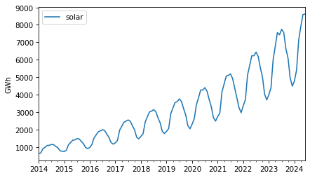
Over this interval, total production has increased several times over. And it’s clear that the magnitude of seasonal variation has increased as well.

If suppose that the magnitudes of seasonal and random variation are proportional to the magnitude of the trend, that suggests an alternative to the additive model in which the time series is the product of a trend, a seasonal component, and a residual component.

To try out this multiplicative model, we’ll split this series into training and test sets.

training, test = split_series(solar)

And call seasonal_decompose with the model=multiplicative argument.

decomposition = seasonal_decompose(training, model="multiplicative", period=12)

Here’s what the results look like.

plot_decomposition(training, decomposition)

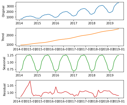
Now the seasonal and residual components are multiplicative factors. So, it looks like the seasonal component varies from about 25% below the trend to 25% above. And the residual component is usually less than 5% either way, with the exception of some larger factors in the first period.

trend = decomposition.trend
seasonal = decomposition.seasonal
resid = decomposition.resid

The R² value of this model is very high.

rsquared = 1 - resid.var() / training.var()
rsquared

0.9999999992978134

The production of a solar panel is almost entirely a function of the sunlight it’s exposed to, so it makes sense that it follows an annual cycle so closely.

To predict the long term trend, we’ll use a quadratic model.

months = range(len(training))
data = pd.DataFrame({"trend": trend, "months": months}).dropna()
results = smf.ols("trend ~ months + I(months**2)", data=data).fit()

In the Patsy formula, the term "I(months**2)" adds a quadratic term to the model, so we don’t have to compute it explicitly. Here are the results.

display_summary(results)

	coef	std err	t	P>|t|	[0.025	0.975]
Intercept	766.1962	13.494	56.782	0.000	739.106	793.286
months	22.2153	0.938	23.673	0.000	20.331	24.099
I(months ** 2)	0.1762	0.014	12.480	0.000	0.148	0.205

R-squared:

0.9983

The p-values of the linear and quadratic terms are very low, which suggests that the quadratic model captures more information about the trend than a linear model would – and the R² value is very high.

Now we can use the model to compute the expected value of the trend for the past and future.

months = range(len(solar))
df = pd.DataFrame({"months": months})
pred_trend = results.predict(df)
pred_trend.index = solar.index

Here’s what it looks like.

pred_trend.plot(color="0.8", label="quadratic model")
trend.plot(color="C1")
decorate(ylabel="GWh")

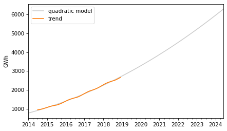
The quadratic model fits the past trend well. Now we can use the seasonal component from the decomposition to predict the seasonal component.

monthly_averages = seasonal.groupby(seasonal.index.month).mean()
pred_seasonal = monthly_averages[pred_trend.index.month]
pred_seasonal.index = pred_trend.index

Finally, to compute “retrodictions” for past values and predictions for the future, we multiply the trend and the seasonal component.

pred = pred_trend * pred_seasonal

Here is the result along with the training data.

training.plot(label="training")
pred.plot(alpha=0.6, color="0.6", label="prediction")
decorate(ylabel="GWh")

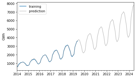
The retrodictions fit the training data well and the predictions seem plausible – now let’s see if they turned out to be accurate. Here are the predictions along with the test data.

future = pred[test.index]
future.plot(ls="--", color="0.6", label="prediction")

test.plot(label="actual")
decorate(ylabel="GWh")

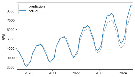
For the first three years, the predictions are very good. After that, it looks like actual growth exceeded expectations.

In this example, seasonal decomposition worked well for modeling and predicting solar production, but in the previous example, it was not very effective for nuclear production. In the next section, we’ll try a different approach, autoregression.