Download the World in Data
Our World in Data recently announced that they are providing APIs to access their data. Coincidentally, I am using one of their datasets in my workshop on time series analysis at PyData Global 2024. So I took this opportunity to update my example using the new API – this notebook shows what I learned.
Click here to run this notebook on Colab. It is based on Chapter 12 of Think Stats, third edition.
import numpy as np
import pandas as pd
import matplotlib.pyplot as plt
Air Temperature
In the chapter on time series analysis, in an exercise on seasonal decomposition, I use monthly average surface temperatures in the United States, from a dataset from Our World in Data that includes “temperature [in Celsius] of the air measured 2 meters above the ground, encompassing land, sea, and in-land water surfaces,” for most countries in the world from 1941 to 2024.
The following cells download and display the metadata that describes the dataset.
import requests

url = (
    "https://ourworldindata.org/grapher/"
    "average-monthly-surface-temperature.metadata.json"
)
query_params = {
    "v": "1",
    "csvType": "full",
    "useColumnShortNames": "true"
}
headers = {'User-Agent': 'Our World In Data data fetch/1.0'}

response = requests.get(url, params=query_params, headers=headers)
metadata = response.json()
The result is a nested dictionary. Here are the top-level keys.
metadata.keys()
dict_keys(['chart', 'columns', 'dateDownloaded'])
Here’s the chart-level documentation.
from pprint import pprint

pprint(metadata['chart'])
{'citation': 'Contains modified Copernicus Climate Change Service information '
             '(2019)',
 'originalChartUrl': 'https://ourworldindata.org/grapher/average-monthly-surface-temperature?v=1&csvType=full&useColumnShortNames=true',
 'selection': ['World'],
 'subtitle': 'The temperature of the air measured 2 meters above the ground, '
             'encompassing land, sea, and in-land water surfaces.',
 'title': 'Average monthly surface temperature'}
And here’s the documentation of the column we’ll use.
pprint(metadata['columns']['temperature_2m'])
{'citationLong': 'Contains modified Copernicus Climate Change Service '
                 'information (2019) – with major processing by Our World in '
                 'Data. “Annual average” [dataset]. Contains modified '
                 'Copernicus Climate Change Service information, “ERA5 monthly '
                 'averaged data on single levels from 1940 to present 2” '
                 '[original data].',
 'citationShort': 'Contains modified Copernicus Climate Change Service '
                  'information (2019) – with major processing by Our World in '
                  'Data',
 'descriptionKey': [],
 'descriptionProcessing': '- Temperature measured in kelvin was converted to '
                          'degrees Celsius (°C) by subtracting 273.15.\n'
                          '\n'
                          '- Initially, the temperature dataset is provided '
                          'with specific coordinates in terms of longitude and '
                          'latitude. To tailor this data to each country, we '
                          'utilize geographical boundaries as defined by the '
                          'World Bank. The method involves trimming the global '
                          'temperature dataset to match the exact geographical '
                          'shape of each country. To correct for potential '
                          "distortions caused by the Earth's curvature on a "
                          'flat map, we apply a latitude-based weighting. This '
                          'step is essential for maintaining accuracy, '
                          'especially in high-latitude regions where '
                          'distortion is more pronounced. The result of this '
                          'process is a latitude-weighted average temperature '
                          'for each nation.\n'
                          '\n'
                          "- It's important to note, however, that due to the "
                          'resolution constraints of the Copernicus dataset, '
                          'this methodology might not be as effective for '
                          'countries with very small landmasses. In these '
                          'cases, the process may not yield reliable data.\n'
                          '\n'
                          '- The derived 2-meter temperature readings for each '
                          'country are calculated based on administrative '
                          'borders, encompassing all land surface types within '
                          'these defined areas. As a result, temperatures over '
                          'oceans and seas are not included in these averages, '
                          'focusing the data primarily on terrestrial '
                          'environments.\n'
                          '\n'
                          '- Global temperature averages and anomalies are '
                          'calculated over all land and ocean surfaces.',
 'descriptionShort': 'The temperature of the air measured 2 meters above the '
                     'ground, encompassing land, sea, and in-land water '
                     'surfaces. The 2024 data is incomplete and was last '
                     'updated 13 October 2024.',
 'fullMetadata': 'https://api.ourworldindata.org/v1/indicators/819532.metadata.json',
 'lastUpdated': '2023-12-20',
 'owidVariableId': 819532,
 'shortName': 'temperature_2m',
 'shortUnit': '°C',
 'timespan': '1940-2024',
 'titleLong': 'Annual average',
 'titleShort': 'Annual average',
 'type': 'Numeric',
 'unit': '°C'}
The following cells download the data for the United States – to see data from another country, change country_code to almost any three-letter ISO 3166 country codes.
country_code = 'USA'    # replace this with other three-letter country codes
base_url = (
    "https://ourworldindata.org/grapher/"
    "average-monthly-surface-temperature.csv"
)

query_params = {
    "v": "1",
    "csvType": "filtered",
    "useColumnShortNames": "true",
    "tab": "chart",
    "country": country_code
}
from urllib.parse import urlencode

url = f"{base_url}?{urlencode(query_params)}"
temp_df = pd.read_csv(url, storage_options=headers)
In general, you can find out which query parameters are supported by exploring the dataset online and pressing the download icon, which displays a URL with query parameters corresponding to the filters you selected by interacting with the chart.
temp_df.head()
| Entity | Code | year | Day | temperature_2m | temperature_2m.1 | |
|---|---|---|---|---|---|---|
| 0 | United States | USA | 1941 | 1941-12-15 | -1.878019 | 8.016244 |
| 1 | United States | USA | 1942 | 1942-01-15 | -4.776551 | 7.848984 |
| 2 | United States | USA | 1942 | 1942-02-15 | -3.870868 | 7.848984 |
| 3 | United States | USA | 1942 | 1942-03-15 | 0.097811 | 7.848984 |
| 4 | United States | USA | 1942 | 1942-04-15 | 7.537291 | 7.848984 |
The resulting DataFrame includes the column that’s documented in the metadata, temperature_2m, and an additional undocumented column, which might be an annual average.
For this example, we’ll use the monthly data.
temp_series = temp_df['temperature_2m']
temp_series.index = pd.to_datetime(temp_df['Day'])
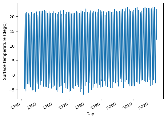
Here’s what it looks like.
temp_series.plot(label=country_code)
plt.ylabel("Surface temperature (℃)");

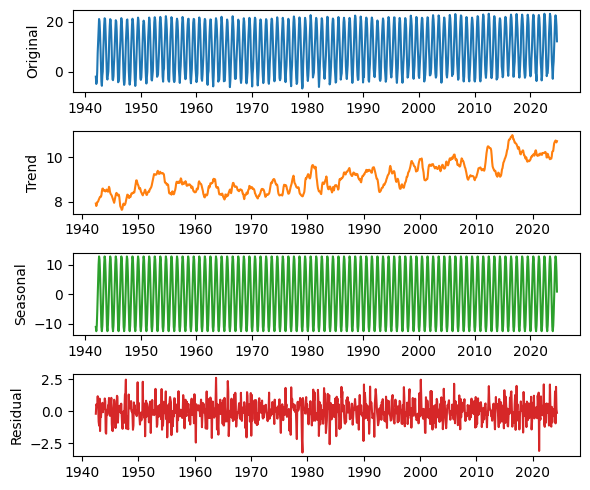
Not surprisingly, there is a strong seasonal pattern. We can use seasonal_decompose from StatsModels to identify a long-term trend, a seasonal component, and a residual.
from statsmodels.tsa.seasonal import seasonal_decompose

decomposition = seasonal_decompose(temp_series, model="additive", period=12)
We’ll use the following function to plot the results.
def plot_decomposition(original, decomposition):
    plt.figure(figsize=(6, 5))

    plt.subplot(4, 1, 1)
    plt.plot(original, label="Original", color="C0")
    plt.ylabel("Original")

    plt.subplot(4, 1, 2)
    plt.plot(decomposition.trend, label="Trend", color="C1")
    plt.ylabel("Trend")

    plt.subplot(4, 1, 3)
    plt.plot(decomposition.seasonal, label="Seasonal", color="C2")
    plt.ylabel("Seasonal")

    plt.subplot(4, 1, 4)
    plt.plot(decomposition.resid, label="Residual", color="C3")
    plt.ylabel("Residual")

    plt.tight_layout()
plot_decomposition(temp_series, decomposition)

As always, I’m grateful to Our World in Data for making datasets like this available, and now easier to use programmatically.