What’s a Chartist?
Recently I heard the word “chartist” for the first time in my life (that I recall). And then later the same day, I heard it again. So that raises two questions:
- What are the chances of going 57 years without hearing a word, and then hearing it twice in one day?
- Also, what’s a chartist?
To answer the second question first, it’s someone who supported chartism, which was “a working-class movement for political reform in the United Kingdom that erupted from 1838 to 1857”, quoth Wikipedia. The name comes from the People’s Charter of 1838, which called for voting rights for unpropertied men, among other reforms.
To answer the first question, we’ll do some Bayesian statistics. My solution is based on a model that’s not very realistic, so we should not take the result too seriously, but it demonstrates some interesting methods, I think. And as you’ll see, there is a connection to Zipf’s law, which I wrote about last week.
Since last week’s post was at the beginner level, I should warn you that this one is more advanced – in rapid succession, it involves the beta distribution, the t distribution, the negative binomial, and the binomial.
This post is based on Think Bayes 2e, which is available from Bookshop.org and Amazon.
Click here to run this notebook on Colab.
Word Frequencies
If you don’t hear a word for more than 50 years, that suggests it is not a common word. We can use Bayes’s theorem to quantify this intuition. First we’ll compute the posterior distribution of the word’s frequency, then the posterior predictive distribution of hearing it again within a day.
Because we have only one piece of data – the time until first appearance – we’ll need a good prior distribution. Which means we’ll need a large, good quality sample of English text. For that, I’ll use a free sample of the COCA dataset from CorpusData.org. The following cells download and read the data.
download("https://www.corpusdata.org/coca/samples/coca-samples-text.zip")
import zipfile


def generate_lines(zip_path="coca-samples-text.zip"):
    with zipfile.ZipFile(zip_path, "r") as zip_file:
        file_list = zip_file.namelist()
        for file_name in file_list:
            with zip_file.open(file_name) as file:
                lines = file.readlines()
                for line in lines:
                    yield (line.decode("utf-8"))
We’ll use a Counter to count the number of times each word appears.
import re
from collections import Counter

pattern = r"[ /\n]+|--"

counter = Counter()
for line in generate_lines():
    words = re.split(pattern, line)[1:]
    counter.update(word.lower() for word in words if word)
The dataset includes about 188,000 unique strings, but not all of them are what we would consider words.
len(counter), counter.total()
(188086, 11503819)
To narrow it down, I’ll remove anything that starts or ends with a non-alphabetical character – so hyphens and apostrophes are allowed in the middle of a word.
for s in list(counter.keys()):
    if not s[0].isalpha() or not s[-1].isalpha():
        del counter[s]
This filter reduces the number of unique words to about 151,000.
num_words = counter.total()
len(counter), num_words
(151414, 8889694)
Of the 50 most common words, all of them have one syllable except number 38. Before you look at the list, can you guess the most common two-syllable word? Here’s a theory about why common words are short.
for i, (word, freq) in enumerate(counter.most_common(50)):
    print(f'{i+1}\t{word}\t{freq}')
1	the	461991
2	to	237929
3	and	231459
4	of	217363
5	a	203302
6	in	153323
7	i	137931
8	that	123818
9	you	109635
10	it	103712
11	is	93996
12	for	78755
13	on	64869
14	was	64388
15	with	59724
16	he	57684
17	this	51879
18	as	51202
19	n't	49291
20	we	47694
21	are	47192
22	have	46963
23	be	46563
24	not	43872
25	but	42434
26	they	42411
27	at	42017
28	do	41568
29	what	35637
30	from	34557
31	his	33578
32	by	32583
33	or	32146
34	she	29945
35	all	29391
36	my	29390
37	an	28580
38	about	27804
39	there	27291
40	so	27081
41	her	26363
42	one	26022
43	had	25656
44	if	25373
45	your	24641
46	me	24551
47	who	23500
48	can	23311
49	their	23221
50	out	22902
There are about 72,000 words that only appear once in the corpus, technically known as hapax legomena.
singletons = [word for (word, freq) in counter.items() if freq == 1]
len(singletons), len(singletons) / counter.total() * 100
(72159, 0.811715228893143)
Here’s a random selection of them. Many are proper names, typos, or other non-words, but some are legitimate but rare words.
np.random.choice(singletons, 100)
array(['laneer', 'emc', 'literature-like', 'tomyworld', 'roald',
       'unreleased', 'basemen', 'kielhau', 'clobber', 'feydeau',
       'symptomless', 'channelmaster', 'v-i', 'tipsha', 'mjlkdroppen',
       'harlots', 'phaetons', 'grlinger', 'naniwa', 'dadian',
       'banafionen', 'ceramaseal', 'vine-covered', 'terrafirmahome.com',
       'hesten', 'undertheorized', 'fantastycznie', 'kaido', 'noughts',
       'hannelie', 'cacoa', 'subelement', 'mestothelioma', 'gut-level',
       'abis', 'potterville', 'quarter-to-quarter', 'lokkii', 'telemed',
       'whitewood', 'dualmode', 'plebiscites', 'loubrutton',
       'off-loading', 'abbot-t-t', 'whackaloons', 'tuinal', 'guyi',
       'samanthalaughs', 'editor-sponsored', 'neurosciences', 'lunched',
       'chicken-and-brisket', 'korekane', 'ruby-colored',
       'double-elimination', 'cornhusker', 'wjounds', 'mendy', 'red.ooh',
       'delighters', 'tuviera', 'spot-lit', 'tuskarr', 'easy-many',
       'timepoint', 'mouthfuls', 'catchy-titled', 'b.l', 'four-ply',
       "sa'ud", 'millenarianism', 'gelder', 'cinnam',
       'documentary-filmmaking', 'huviesen', 'by-gone', 'boy-friend',
       'heartlight', 'farecompare.com', 'nurya', 'overstaying',
       'johnny-turn', 'rashness', 'mestier', 'trivedi', 'koshanska',
       'tremulousness', 'movies-another', 'womenfolks', 'bawdy',
       'all-her-life', 'lakhani', 'screeeeaming', 'marketings', 'girthy',
       'non-discriminatory', 'chumpy', 'resque', 'lysing'], dtype='<U24')
Now let’s see what the distribution of word frequencies looks like.
Zipf’s Law
One way to visualize the distribution is a Zipf plot, which shows the ranks on the x-axis and the frequencies on the y-axis.
freqs = np.array(sorted(counter.values(), reverse=True))
n = len(freqs)
ranks = range(1, n + 1)
Here’s what it looks like on a log-log scale.
plt.plot(ranks, freqs)

decorate(
    title="Zipf plot", xlabel="Rank", ylabel="Frequency", xscale="log", yscale="log"
)
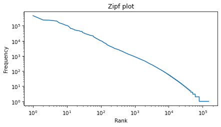
Zipf’s law suggest that the result should be a straight line with slope close to -1. It’s not exactly a straight line, but it’s close, and the slope is about -1.1.
rise = np.log10(freqs[-1]) - np.log10(freqs[0])
rise
-5.664633515191604
run = np.log10(ranks[-1]) - np.log10(ranks[0])
run
5.180166032638616
rise / run
-1.0935235433575892
The Zipf plot is a well-known visual representation of the distribution of frequencies, but for the current problem, we’ll switch to a different representation.
Tail Distribution
Given the number of times each word appear in the corpus, we can compute the rates, which is the number of times we expect each word to appear in a sample of a given size, and the inverse rates, which are the number of words we need to see before we expect a given word to appear.
We will find it most convenient to work with the distribution of inverse rates on a log scale. The first step is to use the observed frequencies to estimate word rates – we’ll estimate the rate at which each word would appear in a random sample.
We’ll do that by creating a beta distribution that represents the posterior distribution of word rates, given the observed frequencies (see this section of Think Bayes) – and then drawing a random sample from the posterior. So words that have the same frequency will not generally have the same inferred rate.
from scipy.stats import beta

np.random.seed(17)
alphas = freqs + 1
betas = num_words - freqs + 1
inferred_rates = beta(alphas, betas).rvs()
Now we can compute the inverse rates, which are the number of words we have to sample before we expect to see each word once.
inverse_rates = 1 / inferred_rates
And here are their magnitudes, expressed as logarithms base 10.
mags = np.log10(inverse_rates)
To represent the distribution of these magnitudes, we’ll use a Surv object, which represents survival functions, but we’ll use a variation of the survival function which is the probability that a randomly-chosen value is greater than or equal to a given quantity. The following function computes this version of a survival function, which is called a tail probability.
from empiricaldist import Surv


def make_surv(seq):
    """Make a non-standard survival function, P(X>=x)"""
    pmf = Pmf.from_seq(seq)
    surv = pmf.make_surv() + pmf

    # correct for numerical error
    surv.iloc[0] = 1
    return Surv(surv)
Here’s how we make the survival function.
surv = make_surv(mags)
And here’s what it looks like.
options = dict(marker=".", ms=2, lw=0.5, label="data")
surv.plot(**options)
decorate(xlabel="Inverse rate (log10 words per appearance)", ylabel="Tail probability")
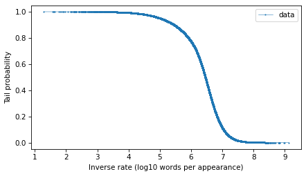
The tail distribution has the sigmoid shape that is characteristic of normal distributions and t distributions, although it is notably asymmetric.
And here’s what the tail probabilities look like on a log-y scale.
surv.plot(**options)
decorate(xlabel="Inverse rate (words per appearance)", yscale="log")
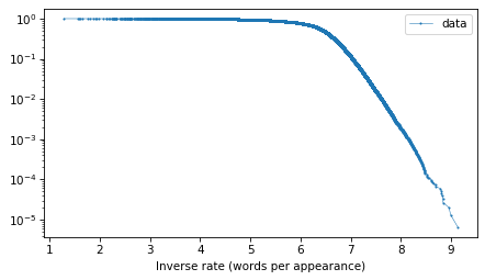
If this distribution were normal, we would expect this curve to drop off with increasing slope. But for the words with the lowest frequencies – that is, the highest inverse rates – it is almost a straight line. And that suggests that a
distribution might be a good model for this data.
Fitting a Model
To estimate the frequency of rare words, we will need to model the tail behavior of this distribution and extrapolate it beyond the data. So let’s fit a t distribution and see how it looks. I’ll use code from Chapter 8 of Probably Overthinking It, which is all about these long-tailed distributions.
The following function makes a Surv object that represents a t distribution with the given parameters.
from scipy.stats import t as t_dist


def truncated_t_sf(qs, df, mu, sigma):
    """Makes Surv object for a t distribution.

    Truncated on the left, assuming all values are greater than min(qs)
    """
    ps = t_dist.sf(qs, df, mu, sigma)
    surv_model = Surv(ps / ps[0], qs)
    return surv_model
If we are given the df parameter, we can use the following function to find the values of mu and sigma that best fit the data, focusing on the central part of the distribution.
from scipy.optimize import least_squares


def fit_truncated_t(df, surv):
    """Given df, find the best values of mu and sigma."""
    low, high = surv.qs.min(), surv.qs.max()
    qs_model = np.linspace(low, high, 2000)
    ps = np.linspace(0.1, 0.8, 20)
    qs = surv.inverse(ps)

    def error_func_t(params, df, surv):
        mu, sigma = params
        surv_model = truncated_t_sf(qs_model, df, mu, sigma)

        error = surv(qs) - surv_model(qs)
        return error

    pmf = surv.make_pmf()
    pmf.normalize()
    params = pmf.mean(), pmf.std()
    res = least_squares(error_func_t, x0=params, args=(df, surv), xtol=1e-3)
    assert res.success
    return res.x
But since we are not given df, we can use the following function to search for the value that best fits the tail of the distribution.
from scipy.optimize import minimize


def minimize_df(df0, surv, bounds=[(1, 1e3)], ps=None):
    low, high = surv.qs.min(), surv.qs.max()
    qs_model = np.linspace(low, high * 1.2, 2000)

    if ps is None:
        t = surv.ps[0], surv.ps[-5]
        low, high = np.log10(t)
        ps = np.logspace(low, high, 30, endpoint=False)

    qs = surv.inverse(ps)

    def error_func_tail(params):
        (df,) = params
        # print(df)
        mu, sigma = fit_truncated_t(df, surv)
        surv_model = truncated_t_sf(qs_model, df, mu, sigma)

        errors = np.log10(surv(qs)) - np.log10(surv_model(qs))
        return np.sum(errors**2)

    params = (df0,)
    res = minimize(error_func_tail, x0=params, bounds=bounds, method="Powell")
    assert res.success
    return res.x
df = minimize_df(25, surv)
df
array([22.52401171])
mu, sigma = fit_truncated_t(df, surv)
df, mu, sigma
(array([22.52401171]), 6.433323515095857, 0.49070837962997577)
Here’s the t distribution that best fits the data.
low, high = surv.qs.min(), surv.qs.max()
qs = np.linspace(low, 10, 2000)
surv_model = truncated_t_sf(qs, df, mu, sigma)
surv_model.plot(color="gray", alpha=0.4, label="model")
surv.plot(**options)
decorate(xlabel="Inverse rate (log10 words per appearance)", ylabel="Tail probability")
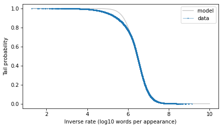
With the y-axis on a linear scale, we can see that the model fits the data reasonably well, except for a range between 5 and 6 – that is for words that appear about 1 time in a million.
Here’s what the model looks like on a log-y scale.
surv_model.plot(color="gray", alpha=0.4, label="model")
surv.plot(**options)
decorate(
    xlabel="Inverse rate (log10 words per appearance)",
    ylabel="Tail probability",
    yscale="log",
)
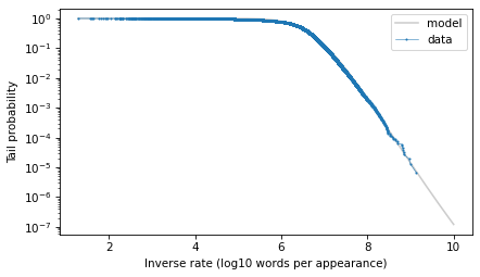
The model fits the data well in the extreme tail, which is exactly where we need it. And we can use the model to extrapolate a little beyond the data, to make sure we cover the range that will turn out to be likely in the scenario where we hear a word for this first time after 50 years.
The Update
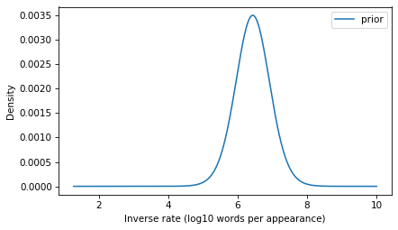
The model we’ve developed is the distribution of inverse rates for the words that appear in the corpus and, by extrapolation, for additional rare words that didn’t appear in the corpus. This distribution will be the prior for the Bayesian update. We just have to convert it from a survival function to a PMF (remembering that these are equivalent representations of the same distribution).
prior = surv_model.make_pmf()
prior.plot(label="prior")
decorate(
    xlabel="Inverse rate (log10 words per appearance)",
    ylabel="Density",
)
To compute the likelihood of the observation, we have to transform the inverse rates to probabilities.
ps = 1 / np.power(10, prior.qs)
Now suppose that in a given day, you read or hear 10,000 words in a context where you would notice if you heard a word for the first time. Here’s the number of words you would hear in 50 years.
words_per_day = 10_000
days = 50 * 365
k = days * words_per_day
k
182500000
Now, what’s the probability that you fail to encounter a word in k attempts and then encounter it on the next attempt? We can answer that with the negative binomial distribution, which computes the probability of getting the nth success after k failures, for a given probability – or in this case, for a sequence of possible probabilities.
from scipy.stats import nbinom

n = 1
likelihood = nbinom.pmf(k, n, ps)
With this likelihood and the prior, we can compute the posterior distribution in the usual way.
posterior = prior * likelihood
posterior.normalize()
1.368245917258196e-11
And here’s what it looks like.
prior.plot(alpha=0.5, label="prior")
posterior.plot(label="posterior")
decorate(
    xlabel="Inverse rate (log10 words per appearance)",
    ylabel="Density",
)
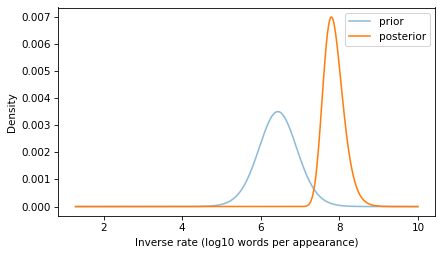
If you go 50 years without hearing a word, that suggests that it is a rare word, and the posterior distribution reflects that logic.
The posterior distribution represents a range of possible values for the inverse rate of the word you heard. Now we can use it to answer the question we started with: what is the probability of hearing the same word again on the same day – that is, within the next 10,000 words you hear?
To answer that, we can use the survival function of the binomial distribution to compute the probability of more than 0 successes in the next n_pred attempts. We’ll compute this probability for each of the ps that correspond to the inverse rates in the posterior.
from scipy.stats import binom

n_pred = words_per_day
ps_pred = binom.sf(0, n_pred, ps)
And we can use the probabilities in the posterior to compute the expected value – by the law of total probability, the result is the probability of hearing the same word again within a day.
p = np.sum(posterior * ps_pred)
p, 1 / p
(0.00016019406802217392, 6242.42840166579)
The result is about 1 in 6000.
With all of the assumptions we made in this calculation, there’s no reason to be more precise than that. And as I mentioned at the beginning, we should probably not take this conclusion too seriously. For one thing, it’s likely that my experience is an example of the frequency illusion, which is “a cognitive bias in which a person notices a specific concept, word, or product more frequently after recently becoming aware of it.” Also, if you hear a word for the first time after 50 years, there’s a good chance the word is having a moment, which greatly increases the chance you’ll hear it again. I can’t think of why chartism might be in the news at the moment, but maybe this post will go viral and make it happen.