Probably Overthinking It

In a previous article, I looked at 93 measurements from the ANSUR-II dataset and found that ear protrusion is not correlated with any other measurement. In a followup article, I used principle component analysis to explore the correlation structure of the measurements, and found that once you have exhausted the information encoded in the most obvious measurements, the ear-related measurements are left standing alone.

I have a conjecture about why ears are weird: ear growth might depend on idiosyncratic details of the developmental environment — so they might be like fingerprints. Recently I discovered a hint that supports my conjecture.

This Veritasium video explains how we locate the source of a sound.

In general, we use small differences between what we hear in each ear — specifically, differences in amplitude, quality, time delay, and phase. That works well if the source of the sound is to the left or right, but not if it’s directly in front, above, or behind — anywhere on vertical plane through the centerline of your head — because in those cases, the paths from the source to the two ears are symmetric.

Fortunately we have another trick that helps in this case. The shape of the outer ear changes the quality of the sound, depending on the direction of the source. The resulting spectral cues makes it possible to locate sources even when they are on the central plane.

The video mentions that owls have asymmetric ears that make this trick particularly effective. Human ears are not as distinctly asymmetric as owl ears, but they are not identical.

And now, based on the Veritasium video, I suspect that might be a feature — the shape of the outer ear might be unpredictably variable because it’s advantageous for our ears to be asymmetric. Almost everything about the way our bodies grow is programmed to be as symmetric as possible, but ears might be programmed to be different.

An article in a recent issue of The Economist suggests, right in the title, “Investors should avoid a new generation of rip-off ETFs”. An ETF is an exchange-traded fund, which holds a collection of assets and trades on an exchange like a single stock. For example, the SPDR S&P 500 ETF Trust (SPY) tracks the S&P 500 index, but unlike traditional index funds, you can buy or sell shares in minutes.

There’s nothing obviously wrong with that – but as an example of a “rip-off ETF”, the article describes “defined-outcome funds” or buffer ETFs, which “offer investors an enviable-sounding opportunity: hold stocks, with protection against falling prices. All they must do is forgo annual returns above a certain level, often 10% or so.”

That might sound good, but the article explains, “Over the long term, they are a terrible deal for investors. Much of the compounding effect of stock ownership comes from rallies.”

To demonstrate, they use the value of the S&P index since 1980: “An investor with returns capped at 10% and protected from losses would have made a real return of 403% over the period, a fraction of the 3,155% return offered by just buying and holding the S&P 500.”

So that sounds bad, but returns from 1980 to the present have been historically unusual. To get a sense of whether buffer ETFs are more generally a bad deal, let’s get a bigger picture.

Click here to run this notebook on Colab

The Dow Jones

The MeasuringWorth Foundation has compiled the value of the Dow Jones Industrial Average at the end of each day from February 16, 1885 to the present, with adjustments at several points to make the values comparable. The series I collected starts on February 16, 1885 and ends on August 30, 2024. The following cells download and read the data.

DATA_PATH = "https://github.com/AllenDowney/ThinkStats/raw/v3/data/"
filename = "DJA.csv"
download(DATA_PATH + filename)

djia = pd.read_csv(filename, skiprows=4, parse_dates=[0], index_col=0)
djia.head()

	DJIA
Date
1885-02-16	30.9226
1885-02-17	31.3365
1885-02-18	31.4744
1885-02-19	31.6765
1885-02-20	31.4252

To compute annual returns, we’ll start by selecting the closing price on the last trading day of each year (dropping 2024 because we don’t have a complete year).

annual = djia.groupby(djia.index.year).last().drop(2024)
annual

	DJIA
Date
1885	39.4859
1886	41.2391
1887	37.7693
1888	39.5866
1889	42.0394
…	…
2019	28538.4400
2020	30606.4800
2021	36338.3000
2022	33147.2500
2023	37689.5400

139 rows × 1 columns

Next we’ll compute the annual price return, which is the ratio of successive year-end closing prices.

annual['Ratio'] = annual['DJIA'] / annual['DJIA'].shift(1)
annual

	DJIA	Ratio
Date
1885	39.4859	NaN
1886	41.2391	1.044401
1887	37.7693	0.915861
1888	39.5866	1.048116
1889	42.0394	1.061960
…	…	…
2019	28538.4400	1.223384
2020	30606.4800	1.072465
2021	36338.3000	1.187275
2022	33147.2500	0.912185
2023	37689.5400	1.137034

139 rows × 2 columns

And the relative return as a percentage.

annual['Return'] = (annual['Ratio'] - 1) * 100

Looking at the years with the biggest losses and gains, we can see that most of the extremes were before the 1960s – with the exception of the 2008 financial crisis.

annual.dropna().sort_values(by='Return')

	DJIA	Ratio	Return
Date
1931	77.9000	0.473326	-52.667396
1907	43.0382	0.622683	-37.731743
2008	8776.3900	0.661629	-33.837097
1930	164.5800	0.662347	-33.765293
1920	71.9500	0.670988	-32.901240
…	…	…	…
1954	404.3900	1.439623	43.962264
1908	63.1104	1.466381	46.638103
1928	300.0000	1.482213	48.221344
1933	99.9000	1.666945	66.694477
1915	99.1500	1.816599	81.659949

138 rows × 3 columns

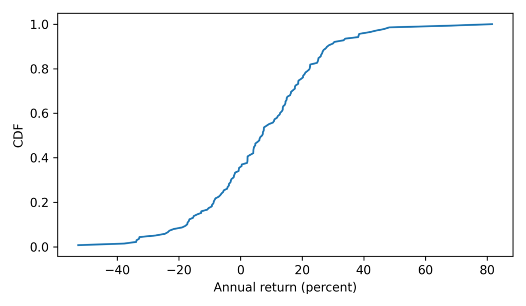
Here’s what the distribution of annual returns looks like.

from empiricaldist import Cdf

cdf_return = Cdf.from_seq(annual['Return'])
cdf_return.plot()

decorate(xlabel='Annual return (percent)', ylabel='CDF')

Immediately we see why capping returns at 10% might be a bad idea – this cap is exceeded almost 45% of the time, and sometimes by a lot!

1 - cdf_return(10)

0.4492753623188406

Long-Term Returns

We’ll use the following function to compute long-term returns. It takes a start date and a duration, and computes two ratios:

• The total price return based on actual annual returns.
• The total price return if annual returns are clipped at 0 and 10 – that is, any negative returns are set to 0 and any returns above 10 are set to 10.

def compute_ratios(start=1993, duration=30):
    end = start + duration
    interval = annual.loc[start: end]
    ratio = interval['Ratio'].prod()
    low, high = 1.0, 1.10
    clipped = interval['Ratio'].clip(low, high)
    ratio_clipped = clipped.prod()
    return start, end, ratio, ratio_clipped

With this function, we can replicate the analysis The Economist did with the S&P 500. Here are the results for the DJIA from the beginning of 1980 to the end of 2023.

compute_ratios(1980, 43)

(1980, 2023, 44.93751117788029, 15.356490985533199)

A buffer ETF over this period would have grown by a factor of more than 15 in nominal dollars, with no risk of loss. But an index fund would have grown by a factor of almost 45. So yeah, the ETF would have been a bad deal.

However, if we go back to the bad old days, an investor in 1900 would have been substantially better off with a buffer ETF held for 43 years – a factor of 7.2 compared to a factor of 2.8.

compute_ratios(1900, 43)

(1900, 1943, 2.8071864303140583, 7.225624631784611)

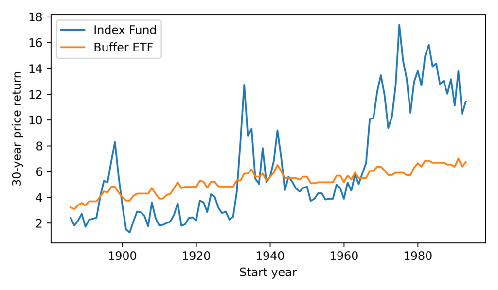
It seems we can cherry-pick the data to make the comparison go either way – so let’s see how things look more generally. Starting in 1886, we’ll compute price returns for all 30-year intervals, ending with the interval from 1993 to 2023.

duration = 30
ratios = [compute_ratios(start, duration) for start in range(1886, 2024-duration)]
ratios = pd.DataFrame(ratios, columns=['Start', 'End', 'Index Fund', 'Buffer ETF'])
ratios.index = ratios['Start']
ratios.tail()

	Start	End	Index Fund	Buffer ETF
Start
1989	1989	2019	13.160027	6.532125
1990	1990	2020	11.116693	6.368615
1991	1991	2021	13.797643	7.005476
1992	1992	2022	10.460407	6.368615
1993	1993	2023	11.417232	6.724757

Here’s what the returns look like for an index fund compared to a buffer ETF.

ratios['Index Fund'].plot()
ratios['Buffer ETF'].plot()

decorate(xlabel='Start year', ylabel='30-year price return')

The buffer ETF performs as advertised, substantially reducing volatility. But it has only occasionally been a good deal, and not in my lifetime.

According to ChatGPT, the primary reasons for strong growth in stock prices since the 1960s are “technological advancements, globalization, financial market innovation, and favorable monetary policies”. If you think these elements will generally persist over the next 30 years, you might want to avoid buffer ETFs.