Probably Overthinking It

Way back in 2013, I wrote this blog post explaining why you should never use a statistical test to check whether a sample came from a Gaussian distribution. I argued that data from the real world never come from a Gaussian distribution, or any other simple mathematical model, so the answer to the question is always no. And there are only two possible outcomes from the test:

• If you have enough data, the test will reject the hypothesis that the data came from a Gaussian distribution, or
• If you don’t have enough data, the test will fail to reject the hypothesis.

Either way, the result doesn’t tell you anything useful.

In this article, I will explore a particular example and demonstrate this relationship between the sample size and the outcome of the test. And I will conclude, again, that

Choosing a distribution is not a statistical question; it is a modeling decision. No statistical test can tell you whether a particular distribution is a good model for your data.

For the technical details, you can read the extended version of this article or run this notebook on Colab.

I’ll start by generating a sample that is actually from a lognormal distribution, then use the sample mean and standard deviation to make a Gaussian model. Here’s what the empirical distribution of the sample looks like compared to the CDF of the Gaussian distribution.

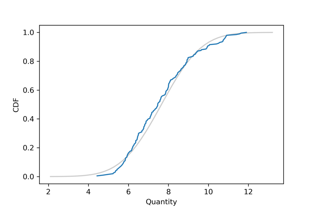
It looks like the Gaussian distribution is a pretty good model for the data, and probably good enough for most purposes.

According to the Anderson-Darling test, the test statistic is 1.7, which exceeds the critical value, 0.77, so at the 5% significance level, we can reject the hypothesis that this sample came from a Gaussian distribution. That’s the right answer, so it might seem like we’ve done something useful. But we haven’t.

Sample size

The result from the A-D test depends on the sample size. The following figure shows the probability of rejecting the null hypothesis as a function of sample size, using the lognormal distribution from the previous section.

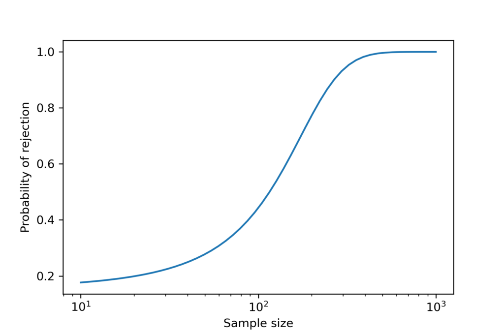
When the sample size is more than 200, the probability of rejection is high. When the sample size is less than 100, the probability of rejection is low. But notice that it doesn’t go all the way to zero, because there is always a 5% chance of a false positive.

The critical value is about 120; at that sample size, the probability of rejecting the null is close to 50%.

So, again, if you have enough data, you’ll reject the null; otherwise you probably won’t. Either way, you learn nothing about the question you really care about, which is whether the Gaussian model is a good enough model of the data for your purposes.

That’s a modeling decision, and no statistical test can help. In the original article, I suggested some methods that might.

A recent question on Reddit asked about using resampling with logistic regression. The responses suggest two ways to do it, one parametric and one non-parametric. I implemented both of them and then invented a third, which is hybrid of the two.

You can read the details of the implementation in the extended version of this article.

Or you can click here to run the Jupyter notebook on Colab

Different ways of computing sampling distributions – and the statistics derived from them, like standard errors and confidence intervals – yield different results. None of them are right or wrong; rather, they are based on different modeling assumptions.

In this example, it is easy to implement multiple models and compare the results. If they were substantially different, we would need to think more carefully about the modeling assumptions they are based on and choose the one we think is the best description of the data-generating process.

But in this example, the differences are small enough that they probably don’t matter in practice. So we are free to choose whichever is easiest to implement, or fastest to compute, or convenient in some other way.

It is a common error to presume that the result of an analytic method is uniquely correct, and that results from computational methods like resampling are approximations to it. Analytic methods are often fast to compute, but they are always based on modeling assumptions and often based on approximations, so they are no more correct than computational methods.

Here’s a question posted on Reddit’s statistics forum:

The Centers for Disease Control and Prevention states on its website that “in the United States, cigarette smoking causes about 90% of lung cancers.” If S is the event “smokes cigarettes” and L is the event “has lung cancer,” then the probability 0.90 is expressed in probability notation as

1. P(S and L).
2. P(S | L).
3. P(L | S).

Let’s consider a scenario that’s not exactly what the question asks about, but will help us understand the relationships among these quantities:

Suppose 20% of people smoke, so out of 1000 people, we have 200 smokers and 800 nonsmokers.

Suppose 1% of nonsmokers get lung cancer, so out of 800 nonsmokers, there would be 8 cases of lung cancer, 0 caused by smoking.

And suppose 20% of smokers get lung cancer, 19% caused by smoking and 1% caused by something else (same as the nonsmokers). Out of 200 smokers, there would be 40 cases of lung cancer, 38 caused by smoking.

In this scenario, there are a total of 48 cases of lung cancer, 38 caused by smoking. So smoking caused 38/48 cancers, which is 79%.

P(S and L) is 40 / 1000, which is 4%.

P(S | L) = 40 / 48, which is 83%.

P(L | S) = 40 / 200, which is 20%.

From this scenario we can conclude:

• The percentage of cases caused by smoking does not correspond to any of the listed probabilities, so the answer to the question is “None of the above”.
• In order to compute these quantities, we need to know the percentage of smokers and the risk ratio for smokers vs nonsmokers.

In reality, the relationships among these quantities are complicated by time: the percentage of smokers changes over time, and there is a long lag between smoking and cancer diagnosis.

Here’s a question from Reddit:

How can I find the least frequent value (antimode) between 2 modes in a bimodal distribution?

I’m only mildly self taught in anything in statistics so please be patient with my ignorance. I’ve found so little info on a Google search for “antimode” that I thought it was a word made up by the author of a random article.

Then I found one tiny mention on the Wikipedia page for “Multimodal distribution” but no citation or details beyond that it’s the least frequent value between modes.

What data do I need in order to find this number and what is the formula?

This site had a short mention of it and in their example listed:

Mode A: 33.25836

Mode B: 71.55446

Antimode: 55.06092

But I can’t seem to reverse engineer it with just this data.

Here’s the reply I wrote:

With continuous data, there is no off-the-shelf formula to compute modes or antimodes. You have to make some modeling decisions.

One option is to use kernel density estimation KDE. Adjust the parameters until, in your judgment, the result is a good representation of the distribution, and then you can read off maxima and minima.

And here’s a notebook on Colab that shows what I mean.

If you are not familiar with KDE, here’s a great animated explanation.